6. Modeling a Single Blade with CAS
In addition to being able to model the blades of the twisted Savonius wind turbine in Geometry Expressions, it is useful to model a single blade in a Computer Algebra System (CAS), such as Maple. In fact, it is actually much easier to create the blade using Maple’s 3D plot feature; however, much less can be done with the blade. In our Geometry Expressions model the surface of the blade is constructed with traces. These traces are parameterized by s and t, where s is the location vertically and t is the location horizontally around the curve of the blade.
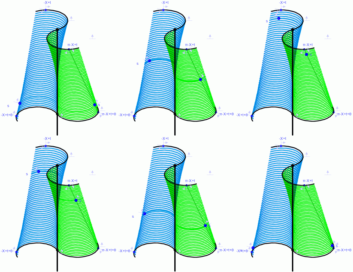
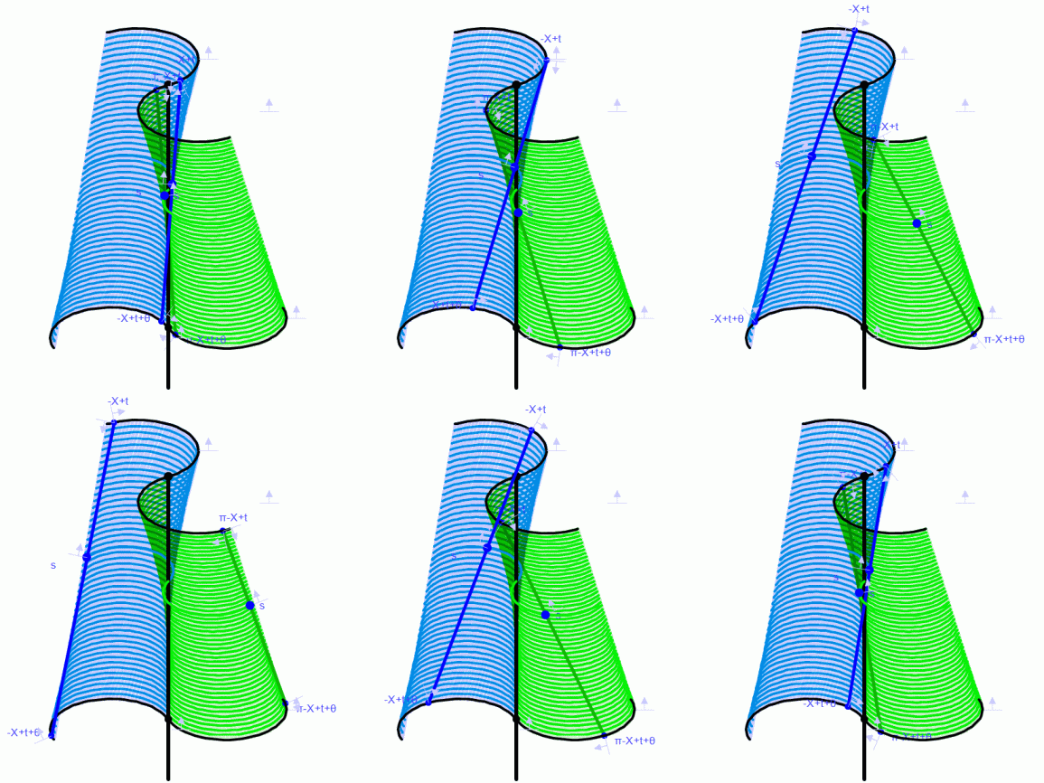
We have one point on our Geometry Expressions model that can be moved to any place on the surface of the blade by varying s and t (see above). If we calculate the symbolic coordinates of these points, we can input them into a Maple 3D Plot and plot the surface of the blade parametrically. The problem, of course, is that our functionally realistic model with cross-pieces has eight of these points. Therefore, Our maple blade will model one of the eight sections, or could model the squeeze again (as in chapter 5). We also need to reduce our equation to having only two variables. Copying the equation from the top view (below) will help with this, because the circles are constrained by r and theta, while the ellipses are constrained by a, b, h, k and theta.
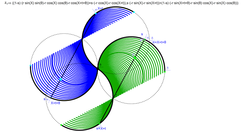
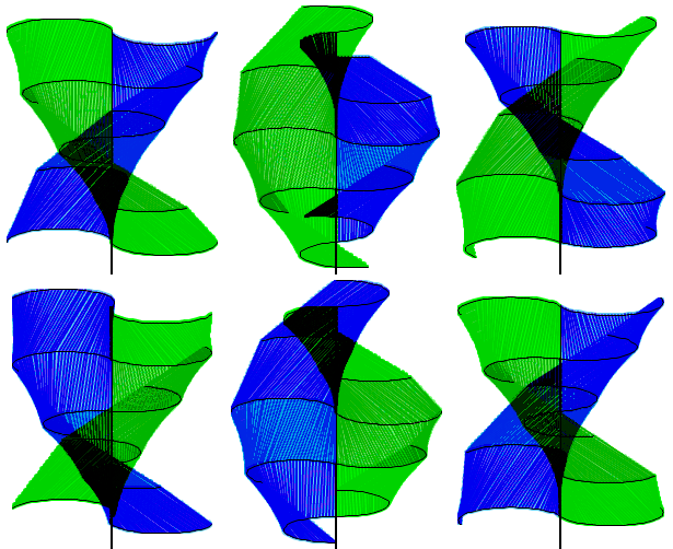
Once we copy our equation (as a maple input) and paste it into maple, we need to add a third term before we can make the 3D plot. Since the point in the top view was represented by X and Y coordinates, we need to add ‘Z’. The Z coordinate is defined by s, but not t, because the purpose of s is to represent the proportion of the way up or down on the turbine the points are. We will multiply s by a constant that will represent the height of the turbine, because otherwise our turbine would only be 1 unit tall. It is easiest to set the radius at 1 and then adjust the constant height accordingly. If this is to be only ¼ of the blade (vertically), then it may be logical for the radius to exceed the height, but this is best determined by eye. We then evaluate the equation for a set value of r and a set value of theta, as well as for X=0 (if your equation had Xs in it). Pi/4 is the most realistic theta value if we are constructing one section of a turbine twisted 180 degrees or pi radians (remember that Maple, and many other CAS, use radians), but you may want to see a bigger twist. Finally, we plot our expression in the interval of our Geometry Expressions traces: t is from 0 to pi and s is from 0 to 1. Our output is a drag-able three-dimensional model of the twisted blade. This is a copy of the Maple worksheet (with dragging motion animation in place of the 3d plots):
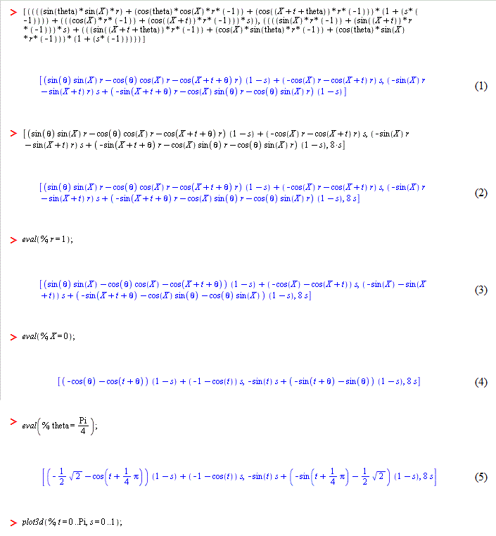

Although this method is a lot faster for modeling the blade and it makes the shape easier to conceptualize, there are many more limitations to this model than our Geometry Expressions one, including the inability to change theta without re-generating the whole image, the inability to stack multiple sections or even create the other blade, and the inability to animate its operation. Therefore, both methods are useful when modeling this shape and we can should use the strengths of each one.
| Previous | Next |
